Rasterizing Pipeline: Supersampling, Antialiasing, Texture Mapping, Mipmaps

Curtis Hu curtisjhu {at} berkeley.edu, Ashvin Verma ashvin.verma {at} berkeley.edu. (February 2025)

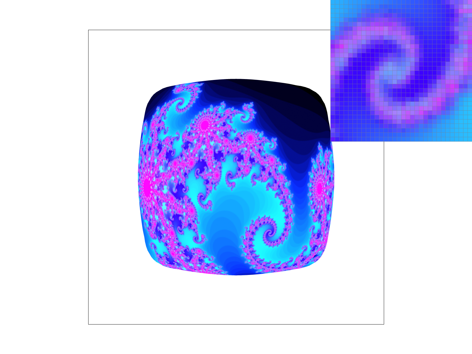
The Julia fractal sampled with different sampling techniques

Drawing Single-Color Triangles

Simple Rasterization

Our first objective for sampling a triangle is to check if a point exists inside the bounds of a triangle. How can we achieve this mathematically?

We can simplify our objective by checking if the point exists on one side of a line. We can do this by defining the right vectors on a line $\overline{AB}$ with point $\textbf{p}$ :

\textbf{N} \cdot \textbf{V} = \text{Perp}(\textbf{B} - \textbf{A}) \cdot (\textbf{p} - \textbf{A})

Here, we are defining the normal vector for $\overline{AB}$ and the vector for $\overline{pA}$ . Intuitively, we can use the properties of dot product to decide which side of the line it is on:

\begin{align*} L_{AB} (\textbf{p}) = \begin{cases} \text{point on the }\textbf{N} \text{ side} \quad \textbf{N} \cdot \textbf{V} < 0 \\ \text{point on opposite } \textbf{N} \text{ side} \quad \textbf{N} \cdot \textbf{V} > 0\\ \text{on line} \quad \textbf{N} \cdot \textbf{V} = 0\\ \end{cases} \end{align*}

We can now do this for all three edges of the triangle and if they are on the same side (assuming our normal vectors are defined consistently), we'll know that $\textbf{p}$ is inside the triangle.

$L_{AB} \text{ and } L_{BC} \text{ and } L_{CA} \text{ are the same side}$ Now to compute our triangle, we can draw a box around the triangle and start iterating all the pixels within. Each pixel location is at the center of the pixel so we have a $(+0.5, +0.5)$ offset with the corners.

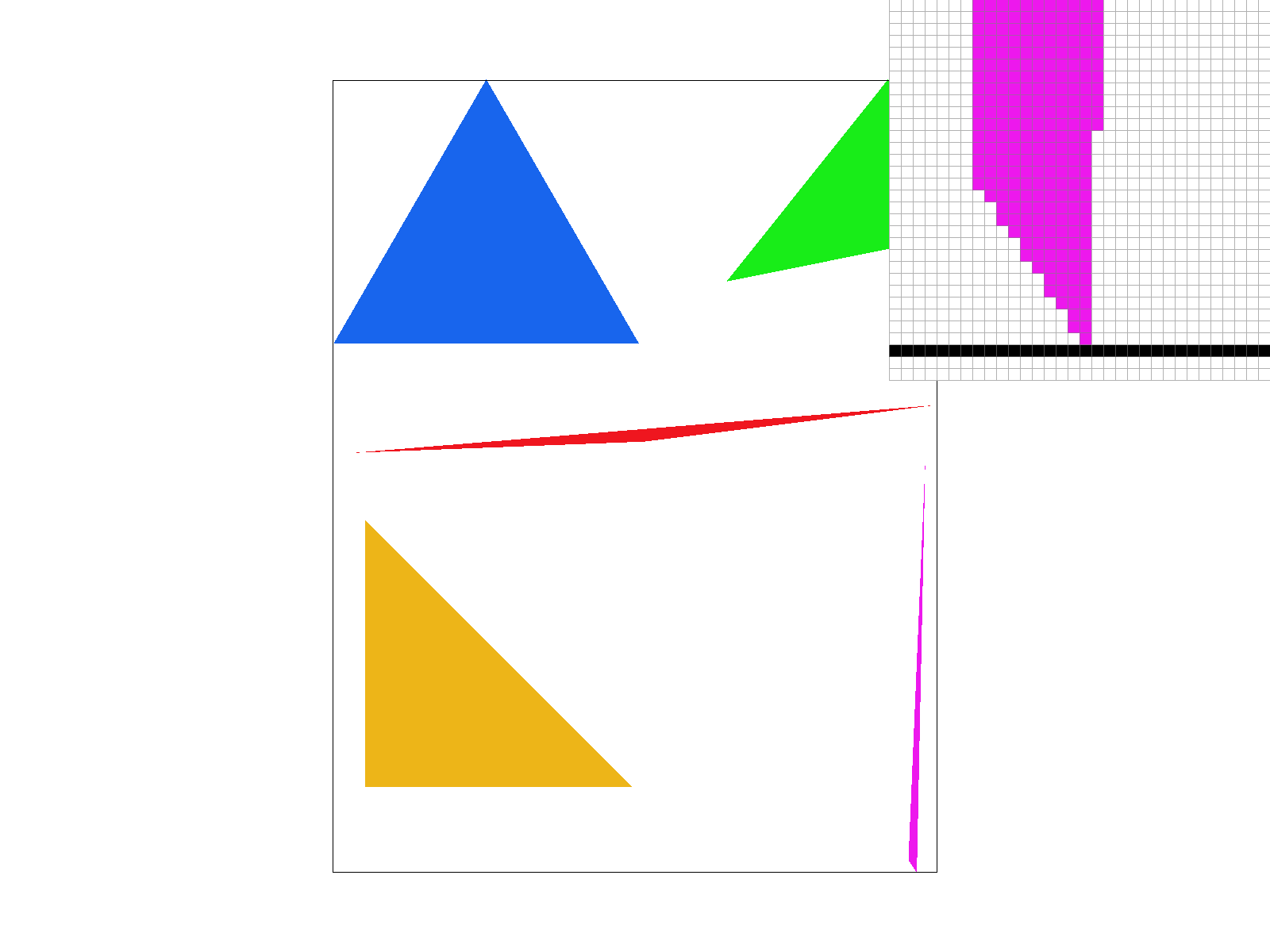
Fig 1. This is the basic rasterizer. For every pixel, we use the algorithm above to decide if that pixel is inside the triangle.

Optimized Solution

As you can probably, tell iterating every pixel within the bounds of the box can be redundant. We can optimize this by iterating only the side lengths of the triangle.

Antialiasing by Supersampling

From Figure 1 above, we can see that there are jaggies (rough edges). Super sampling is useful because it's basically calculating detail at a higher level and averaging/distilling it to a lower-resolution, leading to less jaggies.

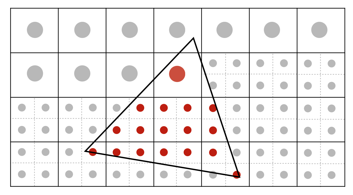
In essence, each pixel is now divided into subpixels. We use the same rasterization for each subpixel. To calculate the shade for the overall pixel, we average the values of these subpixels.

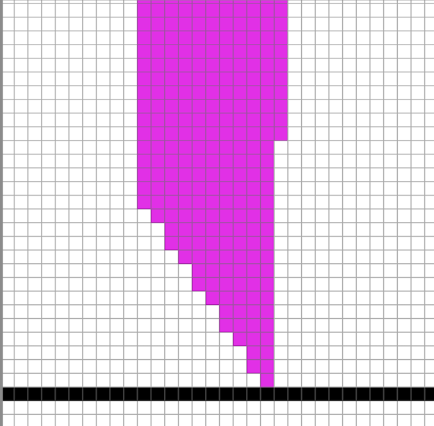
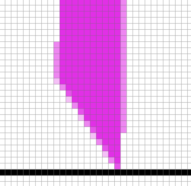
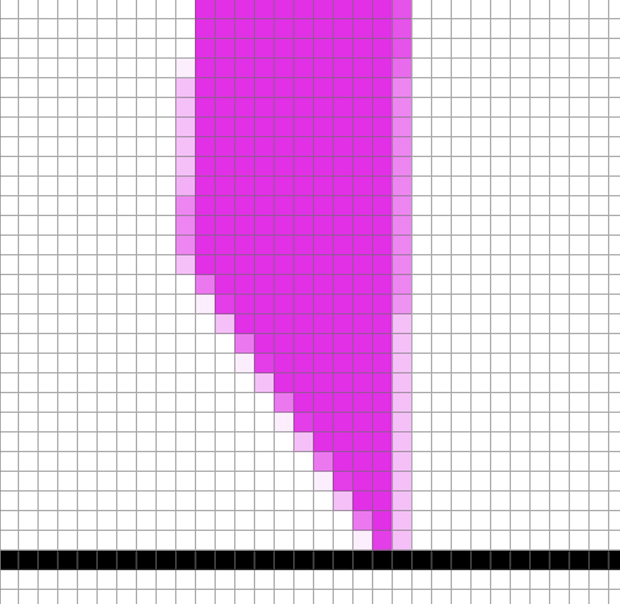
Fig 2. Increasing the sample rate reduces aliasing

Transforms

For transformations, we can use the following "homogenous" vectors:

Points - $(x, y, 1)$ .
Vectors - $(x, y, 0)$

This allows us to distinguish them whilst preserving vector addition between these two classes of vectors. For example, a vector plus point remains a point.

\textbf{Translation} \begin{align*} \begin{bmatrix} 1 & 0 & t_x\\ 0 & 1 & t_y\\ 0 & 0 & 1 \end{bmatrix} \cdot \begin{bmatrix} x\\ y\\ 1 \end{bmatrix} = \begin{bmatrix} x + t_x\\ y + t_y\\ 1 \end{bmatrix} \end{align*}

\textbf{Scaling} \begin{align*} \begin{bmatrix} s_x & 0 & 0\\ 0 & s_y & 0\\ 0 & 0 & 1 \end{bmatrix} \cdot \begin{bmatrix} x\\ y\\ 1 \end{bmatrix} = \begin{bmatrix} s_x x\\ s_y y\\ 1 \end{bmatrix} \end{align*}

\textbf{Rotation} \begin{align*} \begin{bmatrix} \cos\theta & -\sin\theta & 0\\ \sin\theta & \cos\theta & 0\\ 0 & 0 & 1 \end{bmatrix} \cdot \begin{bmatrix} x\\ y\\ 1 \end{bmatrix} \end{align*}

Barycentric coordinates

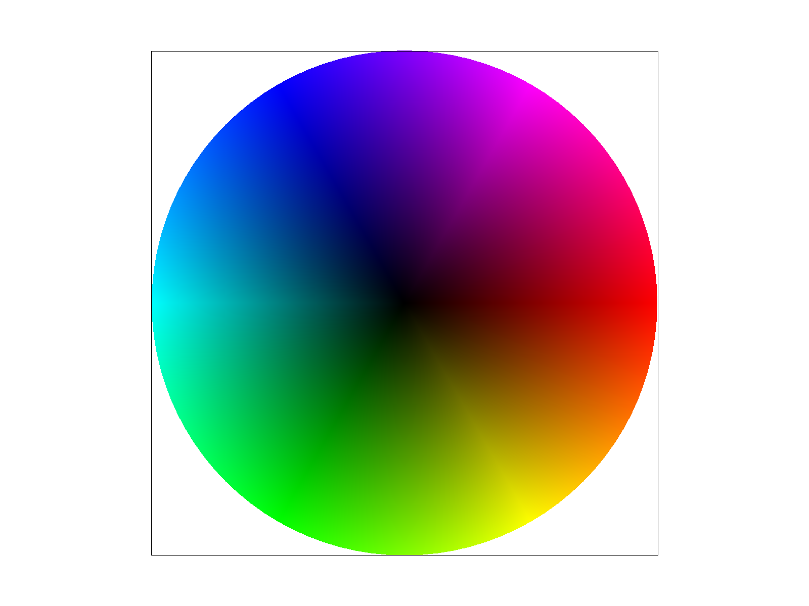
Barycentric coordinates essentially smoothly interpolate between the vertices of a triangle.

More formally, given triangle $\Delta ABC$ , the barycentric coordinate is some linear combination of the vertices:

\begin{align} \textbf{p} &= \alpha \textbf{A} + \beta \textbf{B} + \gamma \textbf{C}\\ 1 &= \alpha + \beta + \gamma \end{align}

As we can see, the point $\textbf{p}$ is some mix between points $\textbf{A}, \textbf{B}, \textbf{C}$

\begin{align*} \alpha &= \frac{L_{BC}(x,y)}{L_{BC}(x_A, y_A)}\\ \beta &= \frac{L_{CA}(x,y)}{L_{CA}(x_B, y_B)}\\ \gamma &= 1 - \alpha - \beta \end{align*}

This is useful since $\alpha, \beta, \gamma$ can interpolate other properties such as RGB colors, pixels on a texture, or better our triangle rasterization algorithm through equation (1). For example, it can make a smooth interpolation of colors found here:

“Pixel sampling” for texture mapping

Say we want to downsample points from an image to display on our screen. How can we best do this to prevent artifacts?

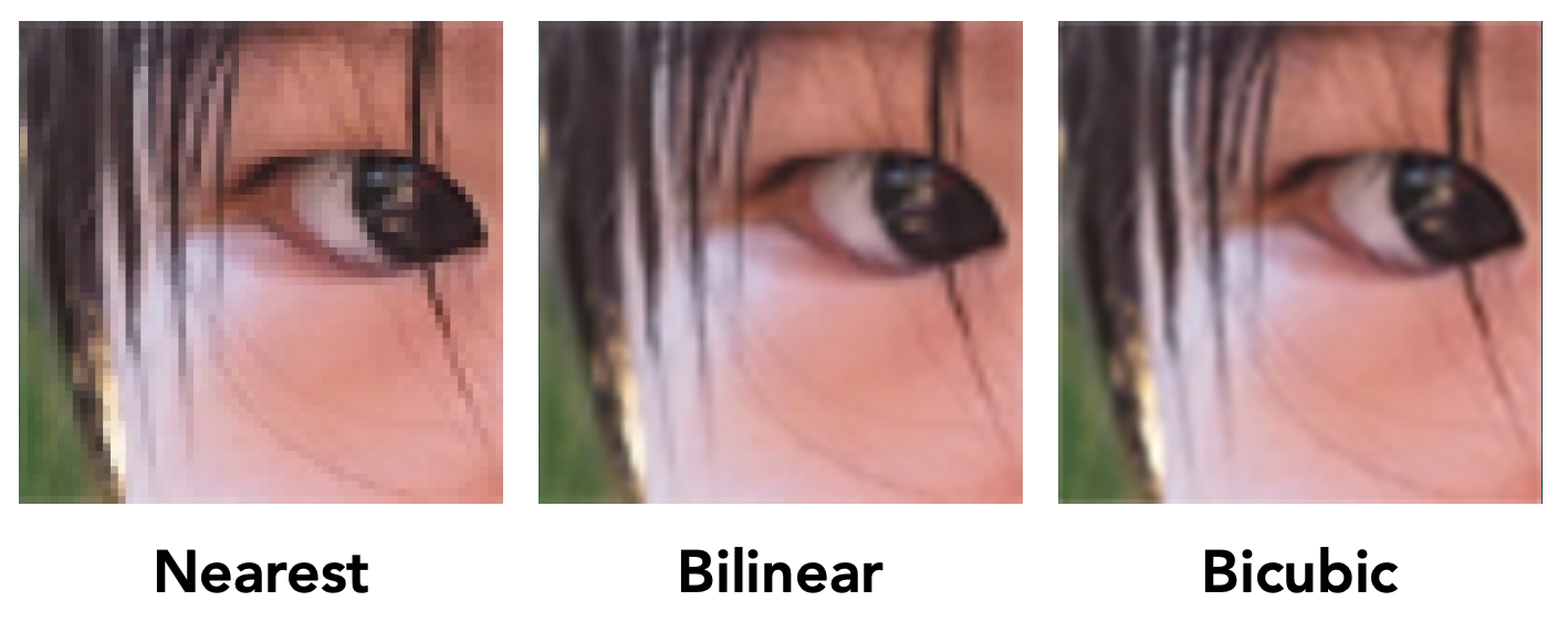
Nearest sampling

In this technique, we map our $xy$ coordinates into $uv$ coordinates and scale it towards the dimensions of the image / texture, then sample the closest pixel in the image / texture.

In layman's terms, we are essentially (using barycentric coordinates) remapping our screen coordinates onto the texture, then finding the pixel coordinates closest to it.

Fig 3. Nearest Sampling at sample rates of 1 and 16

Bilinear sampling

In this technique, we do the same, except linearly interpolate the nearest four pixels in the image.

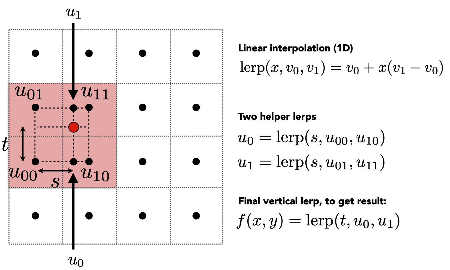
Here, we are using the barycentric coordinates to remap our screen coordinates onto the texture as seen in the red dot above. Instead of just finding the nearest pixel on the texture (which would have been $u_{11}$ ), we linearly interpolate with the closest four pixels. Compared the nearest sampling, we achieve more smoother results.

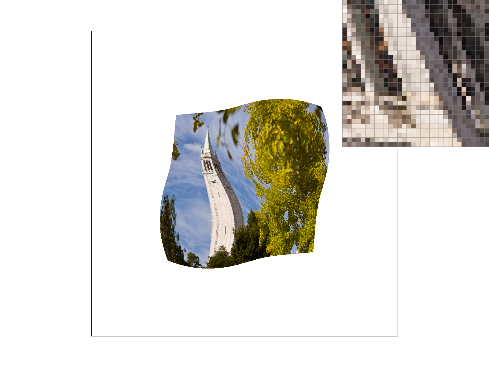
Fig 4. Bilinear Sampling at sample rates of 1 and 16

“Level sampling” with mipmaps for texture mapping

Sometimes, we don't want an even layer of texture mapping. For example, if we are texture mapping over a flat plane, pixels further away will develop jaggies. Instead, we can use mipmap-- lower resolution versions of the image for areas that contain more "warping." Intuitively, if there's a lot of warping, we'll just use a "lower frequency" version of the image so that the "important" information passes through.

While it does solve aliasing, speed and memory are heavily impacted. We'll start calculating the Jacobian matrix which requires calculating two more barycentric points.

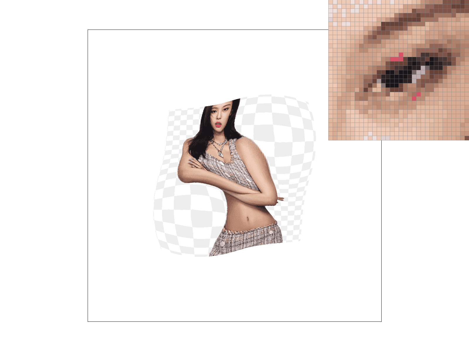
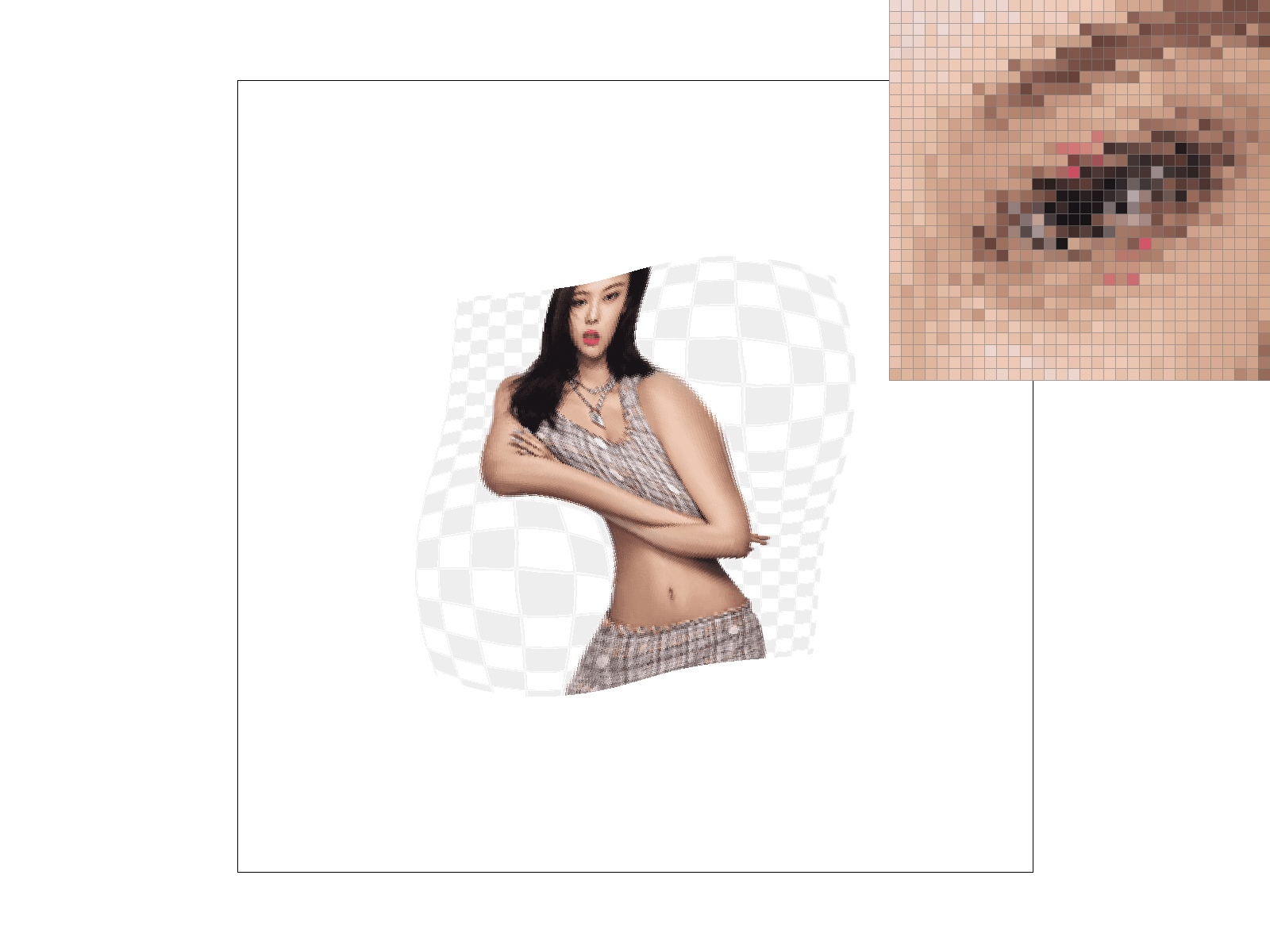
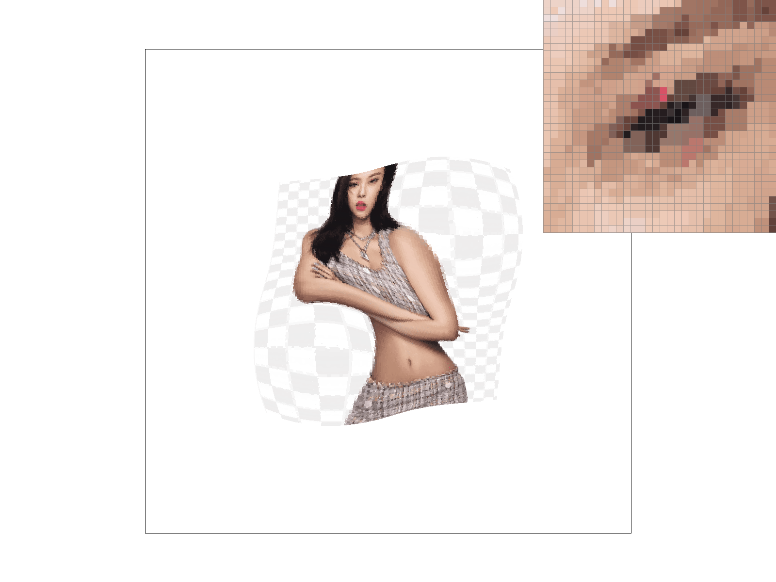
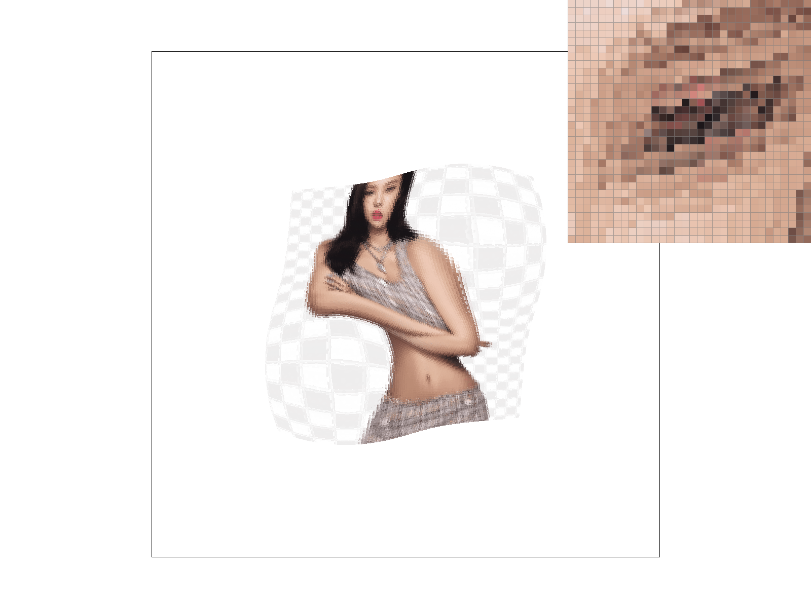
Fig 4. Using different mipmaps

Creative Art!

The following Sierpinski Triangle was rendered with our rasterizer (with the sampling algorithm for triangles)

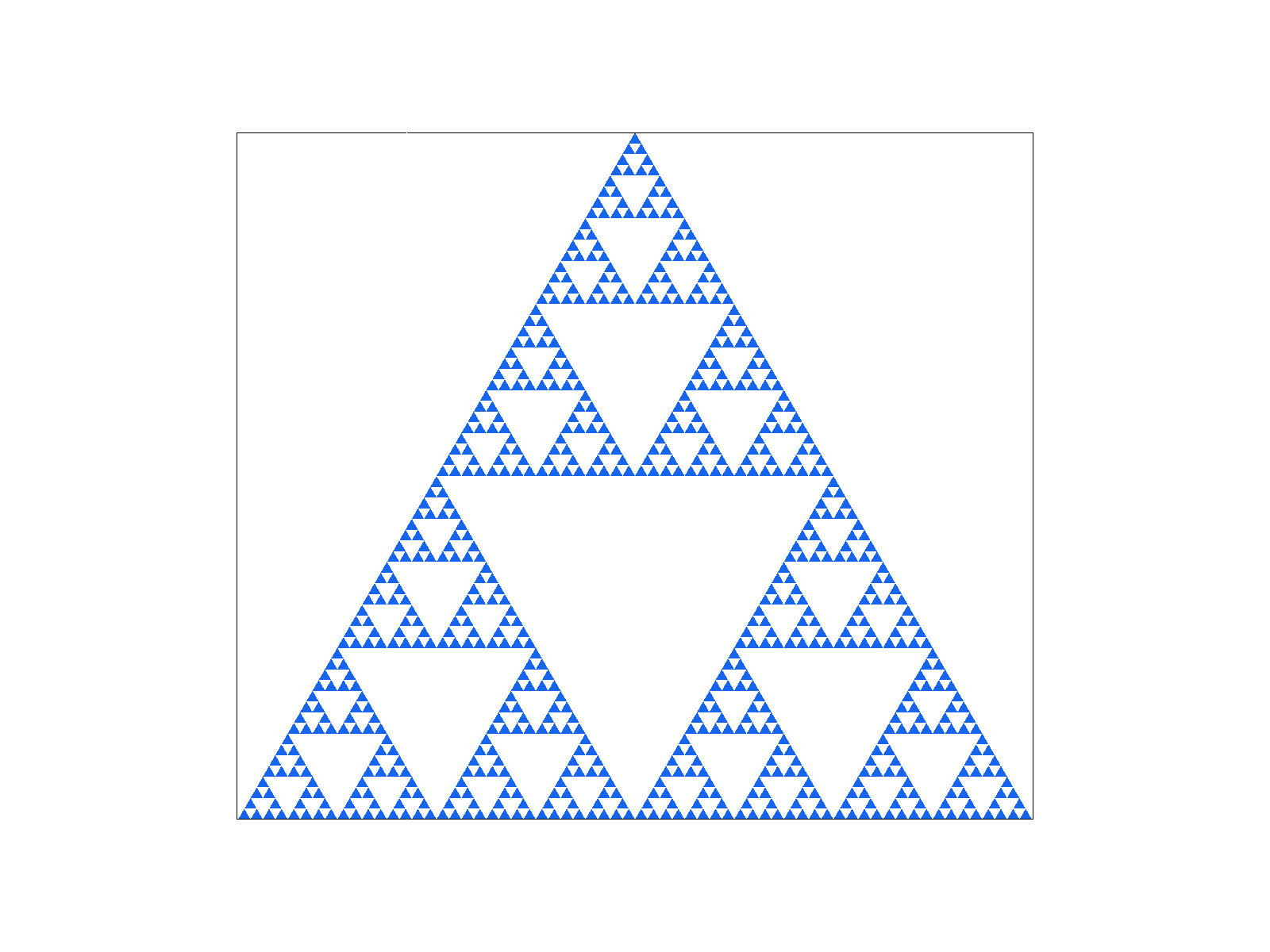
Generated with the following code:

def draw_triangle(x, y, s, level):
    if level == 0:
        x1, y1 = x, y
        x2, y2 = x + s, y
        x3, y3 = x + s/2, y - (s * math.sqrt(3)/2)
        svg_lines.append(f'<polygon points="{x1},{y1} {x2},{y2} {x3},{y3}" />')
    else:
        s_half = s/2
        draw_triangle(x, y, s_half, level-1)
        draw_triangle(x + s_half, y, s_half, level-1)
        draw_triangle(x + s_half/2, y - (s_half * math.sqrt(3)/2), s_half, level-1)

draw_triangle(0, h, size, depth)